Three models, one generator to rule them all
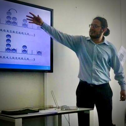
On this page you can run three of the particle systems I work with: independent random walkers, the symmetric exclusion process and the symmetric inclusion process. When we watch them they look very different. Nevertheless, they come from a single formula, in which one parameter selects the model.
We consider particles on a ring of \(L\) sites and denote by \(\eta_x\) the number of particles at site \(x\). A particle at \(x\) jumps to \(y = x + r\) at a rate that depends only on the occupations of the two sites involved. More precisely, the dynamics is given by the generator:
\[ \mathcal L f(\eta) \;=\; \sum_{x}\sum_{r} p(r)\,\eta_x\,(\alpha + \sigma\,\eta_{x+r})\,\big[f(\eta^{x,x+r}) - f(\eta)\big], \]where \(\eta^{x,y}\) denotes the configuration obtained from \(\eta\) by moving one particle from \(x\) to \(y\), and \(p(r) = p(-r)\) is a symmetric jump kernel; in the simulation \(p(r) = 1/(2R)\) for \(1 \le |r| \le R\). The whole interaction sits in the factor \(\alpha + \sigma\,\eta_y\), and the value of \(\sigma\) selects the model:
- \(\sigma = 0\) gives independent random walkers (IRW). The rate \(\alpha\,\eta_x\) does not see the target site, i.e. every particle moves on its own at rate \(\alpha\).
- \(\sigma = -1\) gives the symmetric exclusion process SEP\((\alpha)\). The rate \(\eta_x(\alpha - \eta_y)\) vanishes as soon as \(y\) holds \(\alpha\) particles, hence \(\alpha \in \mathbb N\) is the maximal occupation of a site.
- \(\sigma = +1\) gives the symmetric inclusion process SIP\((\alpha)\). The rate \(\eta_x(\alpha + \eta_y)\) grows with the number of particles already at \(y\): particles attract each other, and the smaller \(\alpha\), the stronger this attraction compared with the free motion.
This unified description is the one we use in our work on higher order fluctuation fields. The same factor also builds the invariant measures: for every density \(\rho\), the product measure whose one-site marginal \(\nu_\rho\) satisfies
\[ \frac{\nu_\rho(k+1)}{\nu_\rho(k)} \;=\; \frac{\alpha + \sigma k}{k+1}\cdot\frac{\rho}{\alpha + \sigma\rho} \]is reversible, i.e. \(\nu_\rho\) is Poisson for IRW, Binomial for SEP and Negative Binomial for SIP.
Pick a model, set the parameters and press play. The panels run together: the particles, their fluctuations around the mean, a space-time picture of the whole history, and the share of particles in the largest pile. The experiments discussed further down can be loaded with the buttons at the end of each section.
Particles
Each dot is a particle, stacked at its site on the ring.
Fluctuations
How far each site is from its mean, \(\eta_x - \mathbb E[\eta_x(t)]\).
One-site law
How many sites hold \(k\) particles.
Space-time
The whole run, from the start (top) to now (bottom). Brighter means more particles.
Largest pile
Shares against \(\log t\).
What to look for
The mean: the three models look the same
Let us start with the average number of particles at a site. Applying the generator to \(\eta_x\), the terms containing \(\sigma\) cancel thanks to the symmetry of \(p\), and we obtain a closed equation:
\[ \frac{d}{dt}\,\mathbb E[\eta_x(t)] \;=\; \alpha \sum_{r} p(r)\,\big(\mathbb E[\eta_{x+r}(t)] - \mathbb E[\eta_x(t)]\big), \]i.e. the mean occupation solves the discrete heat equation for every value of \(\sigma\). This is the gold curve in the particle panel: it is computed exactly from this equation, not from the simulation. Rescaling space by \(L\) and time by \(L^2\), the empirical density converges to the solution of the heat equation \(\partial_t\rho = \tfrac{\chi\alpha}{2}\,\Delta\rho\), with \(\chi = \sum_r r^2 p(r)\). Notice that this hydrodynamic limit does not distinguish independent, exclusion or inclusion particles: at this scale \(\sigma\) is invisible. The white curve is the occupation averaged over a few neighbouring sites, and with many particles per site it follows the gold one closely. While the experiment runs, switch to inclusion particles: the gold curve continues as if nothing had happened.
Fluctuations: where \(\sigma\) appears
The interaction becomes visible as soon as we look at the noise around the mean. Under \(\nu_\rho\) the variance of the occupation of one site is given by:
\[ \operatorname{Var}_{\nu_\rho}(\eta_x) \;=\; \frac{\rho\,(\alpha + \sigma\rho)}{\alpha} \;=\; \rho + \sigma\,\frac{\rho^2}{\alpha}. \]Hence exclusion reduces the noise with respect to independent walkers, and inclusion increases it. In the experiment below \(\rho = 2\) and \(\alpha = 4\), so that the three variances are \(1\), \(2\) and \(3\). The fluctuation panel shows \(\eta_x - \mathbb E[\eta_x(t)]\) together with the band \(\pm 2\sqrt{\rho + \sigma\rho^2/\alpha}\) evaluated at the current mean, and the two numbers above it compare the mean square of the fluctuations with this prediction. The histogram next to it compares the occupations of all sites, averaged over the last few seconds, with the one-site law of the equilibrium on this ring, i.e. with exactly \(N\) particles on \(L\) sites. Switch between the three models while it runs and watch the band and the histogram change.
On large scales these fluctuations are described by the density fluctuation field \(Y^L_t(\varphi) = L^{-1/2}\sum_x \varphi(x/L)\,\big(\eta_x(tL^2) - \rho\big)\). In equilibrium at density \(\rho\) it converges to the Ornstein-Uhlenbeck process solving
\[ dY_t \;=\; \tfrac{\chi\alpha}{2}\,\Delta Y_t\,dt \;+\; \sqrt{\chi\rho\,(\alpha+\sigma\rho)}\;\nabla dW_t, \]where \(W\) is space-time white noise. Once more \(\sigma\) enters only through the factor \(\rho(\alpha + \sigma\rho)\), now in the strength of the noise. In the paper mentioned above we go further, to fields built from orthogonal duality polynomials of higher order in the occupation variables.
Condensation in the inclusion process
For small \(\alpha\) the variance \(\rho + \rho^2/\alpha\) of SIP is much larger than \(\rho^2\), and then a typical site is far from the average. More precisely, the probability of finding a site empty is \(\nu_\rho(0) = (1 + \rho/\alpha)^{-\alpha}\), which tends to one as \(\alpha \to 0\) at fixed \(\rho\): most sites are empty, and the few that are not carry almost all the particles. With \(\rho = 10\) and \(\alpha = 0.01\), about 93% of the sites are empty. This is what we call condensation. On a finite ring the effect is even stronger. With exactly \(N\) particles on \(L\) sites and \(\rho = N/L\), the variance of one site is given by:
\[ \rho\,\Big(1 - \frac1L\Big)\,\frac{\alpha + \sigma\rho}{\alpha + \sigma/L}, \]which for \(\sigma = 1\) and \(\alpha \ll 1/L\) is close to \(\rho^2(L-1)\), i.e. the variance of a configuration with all the particles on a single site.
The difficulty in watching condensation happen is the separation of time scales. Two neighbouring piles of sizes \(\lambda\) and \(\mu\) exchange particles at rate of order \(\lambda\mu\), so starting from an even configuration the piles form after a time of order one. Afterwards a pile only moves when one of its particles leaves, which happens at rate \(\lambda\alpha\), and the new site takes over the whole pile with probability of order \(1/\lambda\). Hence a pile moves at rate of order \(\alpha\), independently of its size, and the piles merge only on times of order \(1/\alpha\) and longer. In the experiment below (\(\alpha = 0.01\)) more than half of the sites are empty by \(t = 10\), while it takes until \(t \approx 10^4\) for the largest pile to hold most of the particles.
A clock running in real time shows either the first phase as a blur or the second one frozen. For this reason the experiment runs on a logarithmic clock: every decade of \(t\) takes the same time on the screen, so that the formation of the piles and their slow merging get the same attention. The time \(t\) displayed above the panels is always the true time of the process. The space-time panel shows the whole story in one picture: many thin lines appear, and then they merge into a few bright ones that wander slowly. The small panel next to it follows the share of particles in the largest pile and the fraction of empty sites, the dashed line being the equilibrium value of the latter. Compare with independent walkers at the same density: the largest pile stays small, and empty sites are exponentially rare.
For two particles, the rigorous counterpart of this picture is our paper Condensation of SIP particles and sticky Brownian motion, where in the regime \(\alpha \to 0\) the distance between two SIP particles converges to a sticky Brownian motion.
How the simulation works
The simulation is exact, in the sense that it samples the Markov process with the generator above without any time discretisation. At every step the next jump \(x \to y\) is chosen with probability proportional to its rate \(p(y-x)\,\eta_x(\alpha + \sigma\eta_y)\), and the clock advances by an exponential time whose parameter is the total rate. The rates of all sites are kept in a binary tree, so that each jump costs of order \(\log L\) operations and a laptop performs several million jumps per second. Everything runs in your browser.